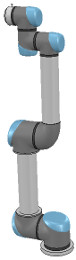
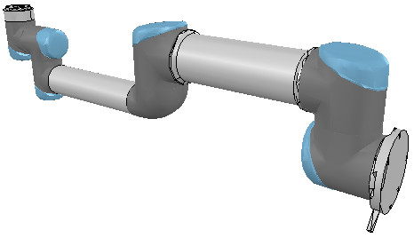
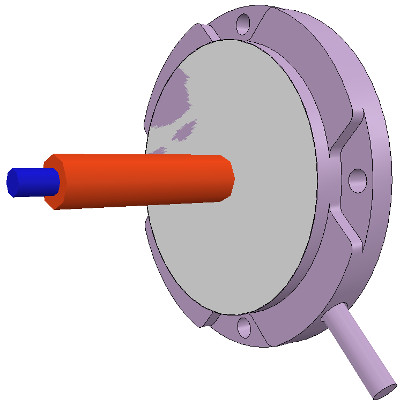
Building a clean model tutorial

This tutorial will guide you step-by-step into building a clean simulation model, of a robot, or any other item. This is a very important topic, maybe the most important aspect, in order to have a nice looking, fast displaying, fast simulating and stable simulation model.

To illustrate the model building process, we will be building following manipulator:

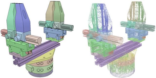
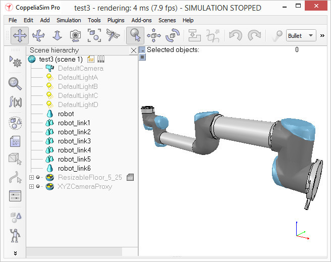
[Model of robotic manipulator]

Building the visible shapes

When building a new model, first, we handle only the visual aspect of it: the dynamic aspect (its undelying even more simplified/optimized model), joints, sensors, etc. will be handled at a later stage.

We could now directly create primitive shapes in CoppeliaSim with [Add > Primitive shape > ...]. When doing this, we have the option to create primitive shapes, or regular shapes. Primitive shapes will be optimized for dynamic interaction, and also directly be dynamically enabled (i.e. fall, collide, but this can be disabled at a later stage). Primitive shapes will be simple meshes, which might not contain enough details or geometric accuracy for our application. Our other option in that case would be to import a mesh from an external application.

When importing CAD data from an external application, the most important is to make sure that the CAD model is not too heavy, i.e. doesn't contain too many triangles. This requirement is important since a heavy model will be slow in display, and also slow down various calculation modules that might be used at a later stage (e.g. minimum distance calculation, or dynamics). Following example is typically a no-go (even if, as we will see later, there are means to simplify the data within CoppeliaSim):

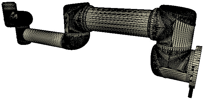
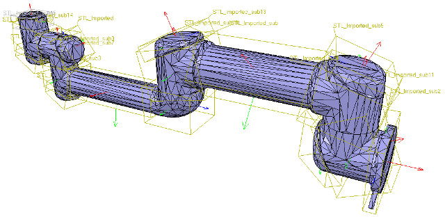
[Complex CAD data (in solid and wireframe)]

Above CAD data is very heavy: it contains many triangles (more than 47'000), which would be ok if we would just use a single instance of it in an empty scene. But most of the time you will want to simulate several instances of a same robot, attach various types of grippers, and maybe have those robots interact with other robots, devices, or the environment. In that case, a simulation scene can quickly become too slow. Generally, we recommend to model a robot with no more than a total of 20'000 triangles, but most of the time 5'000-10'000 triangles would just do fine as well. Remember: less is better, in almost every aspect.

What makes above model so heavy? First, models that contain holes and small details will require much more triangular faces for a correct representation. So, if possible, try to remove all the holes, screws, the inside of objects, etc. from your original model data. If you have the original model data represented as parametric surfaces/objects, then it is most of the time a simple matter of selecting the items and deleting them (e.g. in Solidworks). The second important step is to export the original data with a limited precision: most CAD applications let you specify the level of details of exported meshes. It might also be important to export the objects in several steps, when the drawing consists of large and small objects; this is to avoid having large objects too precisely defined (too many triangles) and small objects too roughly defined (too few triangles): simply export large objects first (by adjusting the desired precision settings), then small objects (by adjusting up precision settings).

Now suppose that we have applied all possible simplifications as described in previous section. We might still end-up with a too heavy mesh after import:

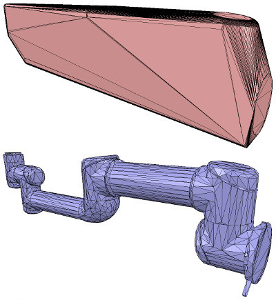
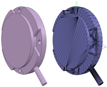
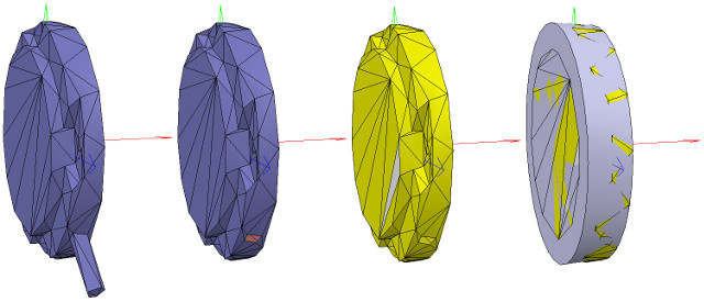
[Imported CAD data]

You can notice that the whole robot was imported as a single mesh. We will see later how to divide it appropriately. Notice also the wrong orientation of the imported mesh: best is to keep the orientation as it is, until the whole model was built, since, if at a later stage we want to import other items that are related to that same robot, they will automatically have the correct position/orientation relative to the original mesh.

At this stage, we have several functions at our disposal, to simplify the mesh:

There is no predefined order in which above functions can/should be applied (except for the first item in the list, which should always be tried first), it heavily depends on the geometry of the mesh we are trying to simplify. Following image illustrates above functions applied to the imported mesh (let's suppose the first item in the list didn't work for us):

[Convex hull, and decimated mesh]

Notice how the convex hull doesn't help us at this stage. We decide to use the mesh decimation function first, and run the function twice in order to divide the number of triangles by a total of 50. We end-up with a mesh containing a total of 2'660 triangles (the original imported mesh contained more than 136'000 triangles!). The number of triangles/vertices a shape contains can be seen in the shape geometry dialog. 2'660 triangles are extremely few triangles for a whole robot model, and the visual appearance might suffer a little bit from it.

At this stage we can start to divide the robot into separate links (remember, we currently have only a single shape for the whole robot). You can do this in two different ways:

In the case of our mesh, method 1 worked fine:

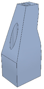
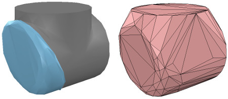
[Divided mesh]

Now, we could further refine/simplify individual shapes. Sometimes also, a shape might look better if its convex hull is used instead. Othertimes, you will have to use several of above's described techniques iteratively, in order to obtain the desired result. Take for instance following mesh:

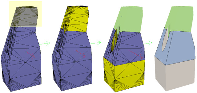
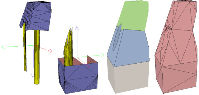
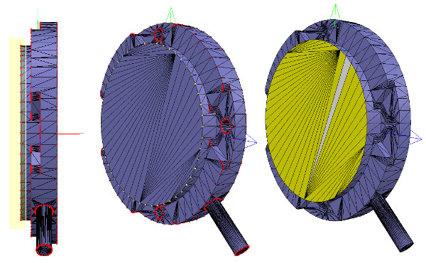
[Imported mesh]

The problem with above's shape is that we cannot simplify it nicely, because of the holes it contains. So we have to go the more complicated way via the shape edit mode, where we can extract individual elements that logically belong to the same convex sub-entity. This process can take several iterations: we first extract 3 approximate convex elements. For now, we ignore the triangles that are part of the two holes. While editing a shape in the shape edit mode, it can be convenient to switch the visibility layers, in order to see what is covered by other scene items.

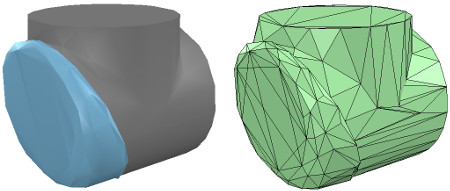
[Step 1]

We end up with a toal of three shapes, but two of them will need further improvement. Now we can erase the triangles that are part of the holes. Finally, we extract the convex hull individually for the 3 shapes, then merge them back together with [Edit > Shape grouping/merging > merge]:

[Step 2]

In CoppeliaSim, we can specify a shading angle that dictates how facetted the shape will display. That parameter, and a few others such as the shape color, can be adjusted in the shape properties. Remember that shapes come in various flavours. In this tutorial we have only dealt with simple shapes up to now: a simple shape has a single set of visual attributes (i.e. one color, one shading angle, etc.). If you merge two shapes, then the result will be a simple shape. You can also group shapes, in which case, each shape will retain its visual attributes.

In next step, we can merge elements that logically belong together (if they are part of the same rigid element, and if they have the same visual attributes). Then we change the visual attributes of the various elements. The easiest ist to adjust a few shapes that have different colors and visual attributes, and if we name the color with a specific string, we can later easily programmatically change that color, also if the shape is part of a compound shape. Then, we select all the shapes that have the same visual attributes, then control-select the shape that was already adjusted, then click Apply to selection, once for the Colors, once for the other properties, in the shape properties: this transfers all visual attributes to the selected shapes (including the color name if you provided one). We end up with 17 individual shapes:

[Adjusted visual attributes]

Now we can group the shapes that are part of the same link with [Edit > Shape grouping/merging > group]. We end up with 7 shapes: the base of the robot (or base of the robot's hierarchy tree), and 6 mobile links. It is also important to correctly name your objects: you we do this with a double-click on the object alias in the scene hierarchy. By defaut, shapes will be assigned to visibility layer 1, but can be changed in the object common properties. By default, only visibility layers 1-8 are activated for the scene. We now have following:

[Individual elements compositn the robot]

When a shape is created or imported, CoppeliaSim will automatically set its reference frame position and bounding box orientation. Both can be changed at any time via [Edit > Shape reference frame > ...] or via [Edit > Shape bounding box> ...]. Select the robot shapes and align their bounding box with the world.

Building the joints

Now we will take care of the joints/motors. Most of the time, we know the exact position and orientation of each of the joints. In that case, we simply add the joints with [Add > Joints > ...], then we can change their position and orientation with the position dialog and orientation dialog. In other situations, we only have the Denavit-Hartenberg (i.e. D-H) parameters. In that case, we can build our joints via the tool model located in Models/tools/Denavit-Hartenberg joint creator.ttm, in the model browser. Othertimes, we have no information about the joint locations and orientations. Then, we need to extract them from the imported mesh. Let's suppose this is our case. Instead of working on the modified, more approximate mesh, we open a new scene, and import the original CAD data again. Most of the time, we can extract meshes or primitive shapes from the original mesh. The first step is to subdivide the original mesh. If that does not work, we do it via the triangle edit mode. Let's suppose that we could divide the original mesh. We now have smaller objects that we can inspect. We are looking for revolute shapes, that could be used as reference to create joints at their locations, with the same orientation. First, remove all objects that are not needed. It is sometimes also useful to work across several opened scenes, for easier visualization/manipulation. In our case, we focus first on the base of the robot: it contains a cylinder that has the correct position for the first joint. In the triangle edit mode, we have:

[Robot base: normal and triangle edit mode visualization]

We change the camera view via the page selector toolbar button, in order to look at the object from the side. The fit-to-view toolbar button can come in handy to correctly frame the object in edition. Then we switch to the vertex edit mode and select all vertices that belong to the upper disc. Remember that by switching some layers on/off, we can hide other objects in the scene. Then we switch back to the triangle edit mode:

[Selected upper disc, vertex edit mode (1 & 2), triangle edit mode (3)]

Now we click Extract cylinder (Extract shape would also work in that case), this just created a cylinder shape in the scene, based on the selected triangles. We leave the edit mode and discard the changes. Now we add a revolute joint with [Add > Joint > Revolute], keep it selected, then control-select the extracted cylinder shape. In the position dialog, on the position tab, we click Apply to selection: this basically copies the x/y/z position of the cylinder to the joint. Both positions are now identical. In the orientation dialog, on the orientation tab, we also click Apply to selection: the orientation of our selected objects is now also the same. Sometimes, we will need to additionally rotate the joint about 90/180 degrees around its own reference frame in order to obtain the correct orientation or rotation direction. We could do that on the rotation tab of that dialog if needed (in that case, do not forget to click the Own frame button). In a similar way we could also shift the joint along its axis, or even do more complex operations. This is what we have:

[Joint in correct location, with the correct orientation]

Now we copy the joint back into our original scene, and save it (do not forget to save your work on a regular basis! The undo/redo function is useful, but doesn't protect you against other mishaps). We repeat above procedure for all the joints in our robot, then rename them. We also make all joints a little bit longer in the joint properties, in order to see them all. By defaut, joints will be assigned to visibility layer 2, but can be changed in the object common properties. We assign now all joints to visibility layer 10, then temporarily enable visibility layer 10 for the scene to also visualize those joints (by default, only visibility layers 1-8 are activated for the scene). This is what we have:

[Joints in correct configuration]

At this point, we could start to build the model hierarchy and finish the model definition. But if we want opur robot to be dynamically enabled, then there is an additional intermediate step:

Building the dynamic shapes

If we want our robot to be dynamically enabled, i.e. react to collisions, fall, etc., then we need to create/configure the shapes appropriately: a shape can be:

Above two points are illustrated here. Respondable shapes should be as simple as possible, in order to allow for a fast and stable simulation. A physics engine will be able to simulate following 5 types of shapes with various degrees of speed and stability:

So the order of preference would be: primitive shapes, convex shapes, and random shapes. Make sure to also read this page. In case of the robot we want to build, we will make the base of the robot as a primitive cylinder, and the other links as convex or convex decomposed shapes.

We could use the dynamically enabled shapes also as the visible parts of the robot, but that would probably not look good enough. So instead, we will build for each visible shape we have created in the first part of the tutorial a dynamically enabled counterpart, which we will keep hidden: the hidden part will represent the dynamic model and be exclusively used by the physics engine, while the visible part will be used for visualization, but also for minimum distance calculations, proximity sensor detections, etc.

We select object robot, copy-and-paste it into a new scene (in order to keep the original model intact) and start the triangle edit mode. If object robot was a compound shape, we would first have had to ungroup it ([Edit > Shape grouping/merging > ungroup]) then merge the individual shapes ([Edit > Shape grouping/merging > merge]) before being able to start the triangle edit mode. Now we select the few triangles that represent the power cable, and erase them. Then we select all triangles in that shape, and click Extract cylinder. We can now leave the edit mode and we have our base object represented as a primitive cylinder:

[Primitive cylinder generation procedure, in the triangle edit mode]

We rename the new shape (with a double-click on its alias in the scene hierarchy) as robot_dyn, assign it to visibility layer 9, then copy it to the original scene. The rest of the links will be modelled as convex shapes, or compound convex shapes. We now select the first mobile link (i.e. object robot_link1) and generate a convex shape from it with [Add > Convex hull of selection]. We rename it to robot_link_dyn1 and assign it to visibility layer 9. When extracting the convex hull doesn't retain enough details of the original shape, then you could still manually extract several convex hulls from its composing elements, then group all the convex hulls with [Edit > Shape grouping/merging > group]. If that appears to be problematic or time consuming, then you can automatically generate a convex decomposed shape with [Edit > Morph into convex decomposed shape(s)...]:

[Original shape, and convex shape pendant]

[Original shape, and convex decomposed shape pendant]

We now repeat the same procedure for all remaining robot links. Once that is done, we attach each visible shape to its corresponding invisible dynamic pendant. We do this by selecting first the visible shape, then via control-click selecting its dynamic pendant then [Edit > Set parent, keep pose(s)]. The same result can be achieved by dragging the visible shape onto its dynamic pendant in the scene hierarchy:

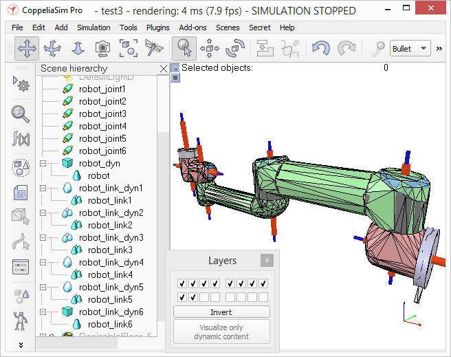
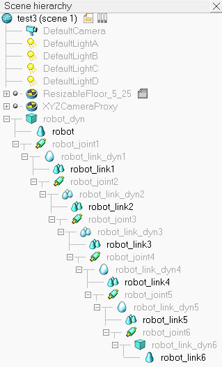
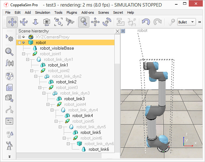
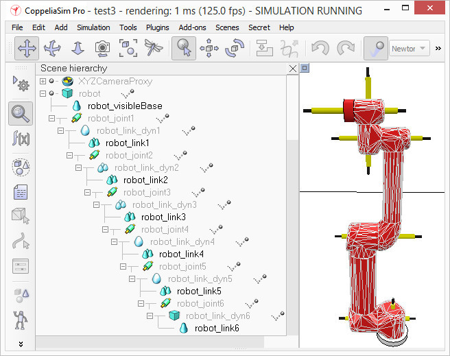
[Visible shapes attached to their dynamic pendants]

We still need to take care of a few things: first, since we want the dynamic shapes only visible to the physics engine, but not to the other calculation modules, we uncheck all object special properties for the dynamic shapes, in the object common properties.

Then, we still have to configure the dynamic shapes as dynamic and respondable. We do this in the shape dynamics properties. Select first the base dynamic shape (i.e. robot_dyn), then check the Body is respondable item. Enable the first 4 Local respondable mask flags, and disable the last 4 Local respondable mask flags: it is important for consecutive respondable links not to collide with each other. For the first mobile dynamic link in our robot (i.e. robot_link_dyn1), we also enable the Body is respondable item, but this time we disable the first 4 Local respondable mask flags, and enable the last 4 Local respondable mask flags. We repeat the above procedure with all other dynamic links, while always alternating the Local respondable mask flags: once the model will be defined, consecutive dynamic shapes of the robot will not generate any collision response when interacting with each other. Try to always end up with a construction where the dynamic base of the robot, and the dynamic last link of the robot have only the first 4 Local respondable mask flags enabled, so that we can attach the robot to a mobile platform, or attach a gripper to the last dynamic link of the robot without dynamic collision interferences.

Finally, we still need to tag our dynamic shapes as Body is dynamic. We do this also in the shape dynamics properties. We can then enter the mass and inertia matrix properties manually, or have those values automatically computed via [Edit > Shape mass and inertia > compute from uniform density...] for selected shapes. Remember also this and that dynamic design considerations. This dynamic base of the robot is a special case: most of the time we want the base of the robot (i.e. robot_dyn) to be non-dynamic (i.e. static), otherwise, if used alone, the robot might fall during movement. But as soon as we attach the base of the robot to a mobile platform, we want the base to become dynamic (i.e. non-static). We do this by enabling the Set to dynamic if gets parent item, then disabling the Body is dynamic item. Now run the simulation: all dynamic shapes, except for the base of the robot, should fall. That attached visual shapes will follow their dynamic pendants.

Model definition

Now we are ready to define our model. We start by building the model herarchy: we attach the last dynamic robot link (robot_link_dyn6) to its corresponding joint (robot_joint6) by selecting robot_link_dyn6, then control-selecting robot_joint6, then [Edit > Set parent, keep pose(s)]. We could also have done this step by simply dragging object robot_link_dyn6 onto robot_link6 in the scene hierarchy. We go on by now attaching robot_joint6 to robot_link_dyn5, and so on, until arrived at the base of the robot. We now have following scene hierarchy:

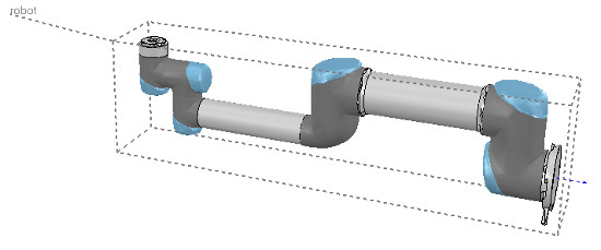
[Robot model hierarchy]

It is nice and more logical to have a simple alias for the model base, since the model base will also represent the model itself. So we rename robot_dyn to robot. Now we select the base of the hierarchy tree (i.e. object robot) and in the object common properties we enable Object is model base. A model bounding box appeared, encompassing the whole robot. The bounding box however appears to be too large: this is because the bounding box also encompasses the invisible items, such as the joints. We now exclude the joints from the model bounding box by enabling the Don't show as inside model selection item for all joints. We could do the same procedure for all invisible items in our model. This is also a useful option in order to also exclude large sensors or other items from the model bounding box. We now have following situation:

[Robot model bounding box]

We now protect our model from accidental modification. We select all visible objects in the robot, then enable Select base of model instead: if we now click a visible link in the scene, the base of the robot will be selected instead. This allows us to manipulate the model as if it was a single object. We can still select visible objects in the robot via control-shift-clicking in the scene, or by selecting the object in the scene hierarchy. We now put the robot into a correct default position/orientation. First, we save current scene as a reference (e.g. if at a later stage we need to import CAD data that have the same orientation at the curent robot). Then we select the model and modify its position/orientation appropriately. It is considered good practice to position the model (i.e. its base object) at X=0 and Y=0.

[Robot model in default configuration]

We now run the simulation: the robot will collapse, since the joints are not controlled by default. When we added the joints in the previous stage, we created joints in dynamic mode, but those are currently not controlled. We can now adjust our joints to our requirements and iIn our case, we want a simple position controller for each one of them. In the joint dynamic properties, we select Position as Control mode. We now run the simulation again: the robot should hold its position. Try to switch the current physics engine to see if the behaviour is consistent across all supported physics engines. You can do this via the appropriate toolbar button, or in the simulation dialog.

During simulation, we now verify the scene dynamic content via the Dynamic content visualization & verification toolbar button. Now, only items that are taken into account by the physics engine will be display, and the display is color-coded. It is very important to always do this, and specially when your dynamic model doesn't behave as expected, in order to quickly debug the model. Similarly, always look at the scene hierarchy during simulation: dynamically enabled objects should display a ball-bounding icon on the right-hand side of their alias.

[Dynamic content visualization & verification]

Finally, we need to prepare the robot so that we can easily attach a gripper to it, or easily attach the robot to a mobile platform (for instance). Two dynamically enabled shapes can be rigidly attached to each other in two different ways:

In our case, only option 2 is of interest. We create a force/torque sensor with [Add > Force sensor], then move it to the tip of the robot, then attach it to object robot_link_dyn6. We change its size and visual appearance appropriately (a red force/torque sensor is often perceived as an optional attachment point, check the various robot models available). We also change its alias to robot_attachment:

[Attachment force/torque sensor]

Now we drag a gripper model into the scene, keep it selected, then control-click the attachment force sensor, then click the Assembling/disassembling toolbar button. The gripper goes into place:

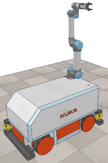
[Attached gripper]

The gripper knew how to attach itself because it was appropriately configured during its model definition. We now also need to properly configure the robot model, so that it will know how to attach itself to a mobile base for instance. We select the robot model, then click Assembling in the object common properties. Set an empty string for 'Parent' match values, then click Set matrix. This will memorize the current base object's local transformation matrix, and use it to position/orient itself relative to the mobile robot's attachment point. To verify that we did things right, we drag the model Models/robots/mobile/KUKA Omnirob.ttm into the scene. Then we select our robot model, then control-click one of the attachment points on the mobile platform, then click the Assembling/disassembling toolbar button. Our robot should correctly place itself on top of the mobile robot:

[Attached robot]

Now we could add additional items to our robot, such as sensors for instance. At some point we might also want to attach embedded scripts to our model, in order to control its behaviour or configure it for various purposes. In that case, make sure to understand how object handles are accessed from embedded scripts. We can also control/access/interface our model from a plugin, from a remote API client, from a ROS node, or from an add-on.

Now we make sure we have reverted the changes done during robot and gripper attachment, we collapse the hierarchy tree of our robot model, select the base of our model, then save it with [File > Save model as...]. If we saved it in the model folder, then the model will be available in the model brower.